Building a 2-layer neural network from scratch with NumPy
In this post we’ll build a two-layer neural network from scratch in Python using only the NumPy library. The full code implementation as well as the test example and plots are contained in this Jupyter notebook.
A two-layer neural network is a parametric function \(f:\mathbb{R}^{m_0} \to \mathbb{R}^{m_2}\) of the form
\[f(\mathbf{x}; \mathbf{W}_1, \mathbf{W}_2, \mathbf{b}_1, \mathbf{b}_2) = \mathbf{W}_2 \sigma(\mathbf{W}_1\mathbf{x} + \mathbf{b}_1) + \mathbf{b}_2 \, .\]The network parameters include the matrices \(\mathbf{W}_1 \in \mathbb{R}^{m_1 \times m_0}\), \(\mathbf{W}_2 \in \mathbb{R}^{m_2 \times m_1}\), which are the weights of the network, and the vectors \(\mathbf{b}_1 \in \mathbb{R}^{m_1}\), \(\mathbf{b}_2 \in \mathbb{R}^{m_2}\), which are the biases. Here \(m_1\) denotes the dimension or number nodes in the hidden layer and the function \(\sigma : \mathbb{R}^{m_1} \to \mathbb{R}^{m_1}\) is an element-wise activation function that allows the network to approximate nonlinear functions.
Given paired training data
\[\texttt{data} = \left\{ \left(\mathbf{x}_i, \mathbf{y}_i \right) \right\}_{i=1}^n\]we want to find parameters \(\mathbf{W}_1,\mathbf{W}_2,\mathbf{b}_1,\mathbf{b}_2\) that minimize the mean-squared error loss function
\[\ell\left(\mathbf{W}_1, \mathbf{W}_2, \mathbf{b}_1, \mathbf{b}_2; \{(\mathbf{x}_i, \mathbf{y}_i) \}_{i=1}^n \right) = \frac{1}{n} \sum_{i=1}^n \lVert f(\mathbf{x}_i) - \mathbf{y}_i\rVert^2\, ,\]so as to fit the network to the data.
Activation function
To finish specifying our network we also need to decide on an activation function. A common choice is the rectified linear unit or ReLU, defined by \(\texttt{relu}(z) = \max(z, 0)\). The ReLU function can easily be implemented using NumPy’s maximum function, which automatically operates element-wise on NumPy arrays.
1
2
3
4
5
     import numpy as np

    def relu(x):
        """Rectified linear activation unit"""
        return np.maximum(x, 0)
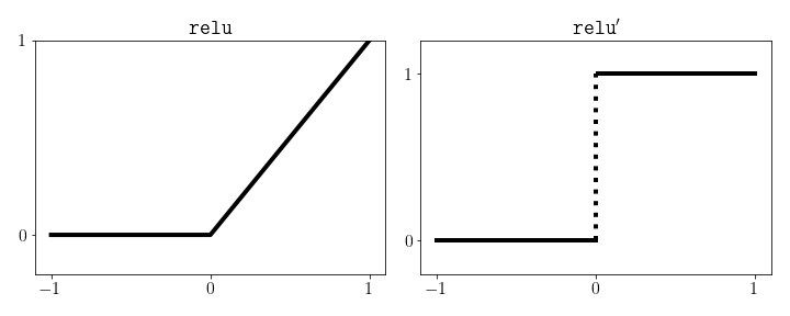
ReLU is differentiable almost everywhere except at the point 0 at which point we need to use a subdifferential. Here we’ll set the derivative at this point to be 0 so that the derivative is the Heaviside function.
\[\texttt{relu}^{\prime}(z) = \begin{cases} 1, & z > 0 \\ 0, & z \le 0 \end{cases}\]Again, this function is easily implemented in NumPy by evaluating a boolean expression at each entry and then casting to a float.
1
2
3
     def grad_relu(x):
        """Heaviside function"""
        return (x > 0).astype(float)
The network class
We’ll implement the two-layer network as a class in Python that contains variables for the parameters as well as functions to predict and train the network. We’ll also add a helper function to compute the loss on the data set as well as evaluate the gradients with respect to the parameters for training. When a network object is instantiated the parameters are initialized to random numbers drawn from a normal distribution.
1
2
3
4
5
6
7
8
9
10
11
12
13
14
15
16
17
18
19
20
21
22
23
     class TwoLayerNetwork:

        def __init__(self, m0, m1, m2):
            """Initialize the network parameters."""
            self.m0 = m0
            self.m1 = m1
            self.m2 = m2
            self.W1 = np.random.randn(m1, m0)
            self.W2 = np.random.randn(m2, m1)
            self.b1 = np.random.randn(m1, 1)
            self.b2 = np.random.randn(m2, 1)

        def predict(self, X):
            """Evaluate the network on the input X."""
            pass

        def grad_loss(self, X, y):
            """Compute the loss and gradients w.r.t. parameters."""
            pass

        def train(self, X, y):
            """Train the network on the data (X, y)."""
            pass
Prediction
The first method we should implement is predict since it is needed to evaluate the function \(f\) on a test input. Let’s suppose that our input vector is a column vector \(\mathbf{x} \in \mathbb{R}^{m_0}\), or equivalently a NumPy array of shape (\(m_0\), 1). For the loss function, we will eventually want to make predictions on a batch of input vectors. Given a batch of training points \(\mathbf{x}_1,\ldots,\mathbf{x}_n \in \mathbb{R}^{m_0}\), define the matrix
so that each input is a column. The output of predict should then be a Numpy array of shape (\(m_2\), \(n\))
where again each column is the corresponding output. It’s convenient to store all of the data in a matrix \(\mathbf{X}\) because matrix multiplication with \(\mathbf{W}_1\) and \(\mathbf{W}_2\) act directly on each column. For example,
\[\mathbf{W}_1\mathbf{X} = \begin{bmatrix} \mathbf{W}_1\mathbf{x}_1 & \cdots & \mathbf{W}_1\mathbf{x}_n \end{bmatrix} \in \mathbb{R}^{m_1 \times n} \, .\]Earlier we also took care to define b1 and b2 as column vectors. This is to ensure that these vectors are correctly added (through NumPy broadcasting) to each column as opposed to the rows in the event that \(m_0 = m_1\).
The code below evaluates the network on a batch of inputs \(\mathbf{X}\) and returns the matrix of outputs \(f(\mathbf{X})\).
1
2
3
4
5
     def predict(self, X):
        """Evaluate the network on test points."""
        y1 = self.W1 @ X + self.b1
        y2 = self.W2 @ relu(y1) + self.b2
        return y2
Loss function and gradients
The next method that we need to implement is a method for computing the loss on the training data as well as the gradient of the loss function with respect to the parameters. This will be critical for training the network and monitoring its performance. To simplify notation as much as possible, let’s define the matrices
\[\mathbf{Y} = \begin{bmatrix} \mathbf{y}_1 & \cdots & \mathbf{y}_n \end{bmatrix} \in \mathbb{R}^{m_2 \times n}\, ,\quad \mathbf{R} = f(\mathbf{X}) - \mathbf{Y} \, .\]The matrix \(\mathbf{R}\) contains the residuals for each point
\[\mathbf{R} = (r_{ji})_{1 \le j \le m_2\\ 1 \le i \le n}\, ,\quad r_{ji} = \left(f(\mathbf{x}_i) - \mathbf{y}_i\right)_j \, ,\]with the subscript \(j\) denoting the row or component of the vector. Because the loss function is the mean-squared error we can write
\[\begin{align*} \texttt{sum}(\mathbf{R} \odot \mathbf{R}) &= \sum_{i=1}^n \sum_{j=1}^{m_2} r_{ji}^2 \\ &= \sum_{i=1}^n \lVert f(\mathbf{x}_i) - \mathbf{y}_i \rVert^2 \\ &= n \cdot \ell\left(\mathbf{W}_1, \mathbf{W}_2, \mathbf{b}_1, \mathbf{b}_2; \{(\mathbf{x}_i, \mathbf{y}_i) \}_{i=1}^n \right) \, , \end{align*}\]where \(\odot\) represents element-wise multiplication and \(\texttt{sum}\) is a function that sums all of the entries in the matrix. In code this looks like:
1
2
3
4
5
6
 def grad_loss(self, X, y):
    """Compute the loss and gradients w.r.t. parameters."""
    n = X.shape[1]
    fx = self.predict(X)
    R = fx - y
    loss = np.sum(R * R)/n
To obtain the gradients of the loss function we will compute them explicitly. For more complicated networks it would be better to use an automatic differentiation package such as Jax or PyTorch, but here the problem is simple enough for us to derive the gradients by hand. For the gradients we get
\begin{align*} \nabla_{\mathbf{W}_1} \ell &= \frac{2}{n} \sum_{i=1}^n \left( \mathbf{W}_2^{\top}\left( f(\mathbf{x}_i) - \mathbf{y}_i\right) \odot \sigma^{\prime}(\mathbf{W}_1\mathbf{x}_i + \mathbf{b}_1) \right) \mathbf{x}_i^{\top} \\ \nabla_{\mathbf{W}_2} \ell &= \frac{2}{n}\sum_{i=1}^n \left( f(\mathbf{x}_i) - \mathbf{y}_i \right) \sigma\left( \mathbf{W}_1\mathbf{x}_i + \mathbf{b}_1\right)^{\top} \\ \nabla_{\mathbf{b}_1} \ell &= \frac{2}{n}\sum_{i=1}^n \mathbf{W}_2^{\top}\left(f(\mathbf{x}_i) - \mathbf{y}_i \right) \odot \sigma^{\prime}(\mathbf{W}_1\mathbf{x}_i + \mathbf{b}_1) \\ \nabla_{\mathbf{b}_2} \ell &= \frac{2}{n}\sum_{i=1}^n \left( f(\mathbf{x}_i) - \mathbf{y}_i \right) \, . \end{align*}
A detailed derivation of these gradients can be found here.
To implement these in Python for a batch of training points and to avoid redundant computations define the matrices
\[\mathbf{S} = \sigma\left( \mathbf{W}_1\mathbf{X} + \mathbf{b}_1 \mathbf{1}_{n}^{\top} \right)\, ,\quad \mathbf{D} = \sigma^{\prime}\left( \mathbf{W}_1\mathbf{X} + \mathbf{b}_1 \mathbf{1}_{n}^{\top} \right) \, ,\]both of which are \(m_1 \times n\) matrices. Here \(\mathbf{1}_n = [1,\ldots, 1] \in \mathbb{R}^{n}\) is a vector of only ones so that
\[\mathbf{b}_1 \mathbf{1}_{n}^{\top} = \begin{bmatrix} \mathbf{b}_1 & \cdots & \mathbf{b}_1 \end{bmatrix} \in \mathbb{R}^{m_1 \times n} \, .\]In Python we don’t actually need to do this because NumPy will automatically broadcast and add the vector \(\mathbf{b}_1\) to each column of the matrix \(\mathbf{W}_1\mathbf{X}\).
1
2
 S = relu(self.W1 @ X + self.b1)
D = grad_relu(self.W1 @ X + self.b1)
We’ll also define the matrix
\[\mathbf{V} = \mathbf{W}_2^{\top}\mathbf{R} \in \mathbb{R}^{m_1 \times n}\, .\]The vectorized implementation of the gradients can be written as
\begin{align*} \nabla_{\mathbf{W}_1} \ell &= \frac{2}{n} \left( \mathbf{V}\odot \mathbf{D} \right) \mathbf{X}^{\top} \\ \nabla_{\mathbf{W}_2} \ell &= \frac{2}{n} \mathbf{R} \mathbf{S}^{\top} \\ \nabla_{\mathbf{b}_1} \ell &= \frac{2}{n}\texttt{sum}\left( \mathbf{V}\odot \mathbf{D},\ \texttt{columns} \right) \\ \nabla_{\mathbf{b}_2} \ell &= \frac{2}{n}\texttt{sum}\left( \mathbf{R},\ \texttt{columns} \right)\, , \end{align*}
where the function \(\texttt{sum}\left( \mathbf{A},\ \texttt{columns} \right)\) denotes the vector that is the sum of the columns of the matrix \(\mathbf{A}\).
Equivalently with NumPy:
1
2
3
4
5
 V = self.W2.T @ R
grad_W1 = (2/n) * (V * D) @ X.T
grad_W2 = (2/n) * (R @ S.T)
grad_b1 = 2 * np.mean(V * D, axis=1)
grad_b2 = 2 * np.mean(R, axis=1)
The complete grad_loss method is below. Note that after computing the gradients grad_b1 and grad_b2 we reshape the Numpy arrays to column vectors to ensure that they are broadcasted correctly. We also use Numpy’s mean function as opposed to the sum function and then dividing by \(n\), in case of potential overflow.
1
2
3
4
5
6
7
8
9
10
11
12
13
14
15
16
17
18
19
20
21
22
23
24
25
26
27
 def grad_loss(self, X, y):
    """Compute the gradient of the loss on the training set."""
    n = X.shape[1]  # Number of training samples
    fx = self.predict(X)  # shape (m2, n)

    # Pre-compute matrices
    R = fx - y # residuals
    V = self.W2.T @ R
    S = relu(self.W1 @ X + self.b1) # shape (m1, n)
    D = grad_relu(self.W1 @ X + self.b1) # shape (m1, n)

    # Multiply the loss by m2 since there are n*m2 elements
    # in the matrices fx, y
    loss = self.m2 * np.mean(R*R)

    # Gradients
    grad_W1 = (2/n) * (V * D) @ X.T

    grad_W2 = (2/n) * (R @ S.T)

    grad_b1 = 2 * np.mean(V * D, axis=1)
    grad_b1 = grad_b1.reshape((self.m1, 1))

    grad_b2 = 2 * np.mean(R, axis=1)
    grad_b2 = grad_b2.reshape((self.m2, 1))

    return loss, grad_W1, grad_W2, grad_b1, grad_b2
Training
Now that the gradients are implemented we can use gradient descent to train the network. We will keep the training method as simple by specifying a fixed learning rate and a fixed number of epochs. We will also use full gradient descent as opposed to stochastic gradient descent or minibatches.
1
2
3
4
5
6
7
8
9
10
11
12
13
 def train(self, Xtrain, ytrain, lr, epochs):
    """Train the network using gradient descent."""
    for t in range(epochs):
        # Compute loss function and gradients
        loss, grad_W1, grad_W2, grad_b1, grad_b2 = \
        self.grad_loss(Xtrain, ytrain)

        # Update parameters
        self.W1 -= lr*grad_W1
        self.W2 -= lr*grad_W2
        self.b1 -= lr*grad_b1
        self.b2 -= lr*grad_b2
    return loss
Completed network class
Note that in the train method we also use the tqdm package to track the optimizer’s progress.
1
2
3
4
5
6
7
8
9
10
11
12
13
14
15
16
17
18
19
20
21
22
23
24
25
26
27
28
29
30
31
32
33
34
35
36
37
38
39
40
41
42
43
44
45
46
47
48
49
50
51
52
53
54
55
56
57
58
59
60
61
62
63
64
65
66
67
68
69
70
71
72
73
74
75
76
77
78
79
80
81
82
83
84
85
86
87
88
89
90
91
92
93
94
95
96
97
98
99
100
101
102
103
104
105
106
107
108
109
110
111
112
113
114
115
116
117
118
119
120
121
122
123
124
125
126
127
128
129
130
131
132
133
134
135
136
137
138
 import numpy as np
from tqdm import tqdm


def relu(x):
    """Rectified linear unit

    Input:
    x - numpy array of shape (m, n) where n is the number
        of points and m is the dimension

    Return:
    numpy array of shape (m ,n) of the pointwise ReLU
    """
    return np.maximum(x, 0)


def grad_relu(x):
    """Heaviside function

    Input:
    x - numpy array of shape (m, n) where n is the number
        of points and m is the dimension

    Return:
    numpy array of shape (m ,n) of the pointwise Heaviside
    """
    return (x > 0).astype(float)


class TwoLayerNetwork:

    def __init__(self, m0, m1, m2):
        """Initialize the network with random weights.

        Input:
        m0 - int for the input dimension
        m1 - int for the hidden layer dimension
        m2 - int for the output dimension
        """
        self.m0 = m0
        self.m1 = m1
        self.m2 = m2
        # Weight matrices
        self.W1 = np.random.randn(m1, m0)
        self.W2 = np.random.randn(m2, m1)
        # Save b1, b2 as column vectors for correct
        # broadcasting during prediction.
        self.b1 = np.random.randn(m1, 1)
        self.b2 = np.random.randn(m2, 1)


    def predict(self, X):
        """Evaluate the network on test points.

        Input:
        X - numpy array of shape (m0, n) where m0 is the input
            dimension and n is the number of points

        Return:
        y2 - numpy array of shape (m2, n) where m2 is the
             output dimension of the network
        """
        y1 = self.W1 @ X + self.b1
        y2 = self.W2 @ relu(y1) + self.b2
        return y2


    def grad_loss(self, X, y):
        """Compute the gradient of the loss on the training set.

        The loss is given by
        1/n sum_{i=1}^n ||f(x_i) - y_i||^2

        Input:
        X - numpy array of shape (m0, n)
        y - numpy array of shape (m2, n)

        Return:
        loss - float for the mean-squared error of the network on
               the training points
        grad_W1 - numpy array of shape (m0, m1)
        grad_W2 - numpy array of shape (m1, m2)
        grad_b1 - numpy array of shape (m1, 1)
        grad_b2 - numpy array of shape (m2, 1)
        """
        n = X.shape[1]  # Number of training samples
        fx = self.predict(X)  # shape (m2, n)

        # Pre-compute matrices
        R = fx - y # residuals
        V = self.W2.T @ R
        S = relu(self.W1 @ X + self.b1) # shape (m1, n)
        D = grad_relu(self.W1 @ X + self.b1) # shape (m1, n)

        # Multiply the loss by m2 since there are n*m2 elements
        # in the matrices fx, y
        loss = self.m2 * np.mean(R*R)

        # Gradients
        grad_W1 = (2/n) * (V * D) @ X.T

        grad_W2 = (2/n) * (R @ S.T)

        grad_b1 = 2 * np.mean(V * D, axis=1)
        grad_b1 = grad_b1.reshape((self.m1, 1))

        grad_b2 = 2 * np.mean(R, axis=1)
        grad_b2 = grad_b2.reshape((self.m2, 1))

        return loss, grad_W1, grad_W2, grad_b1, grad_b2


    def train(self, X, y, lr, epochs):
        """Train the network using gradient descent.
        Updates the network parameters in place.

        Input:
        X - numpy array of shape (m0, n)
        y - numpy array of shape (m2, n)
        lr - float > 0 that specifies the learning rate
        epochs - int > 0 that specifies the number of iterations

        Return:
        loss - float for the final mean-squared error of the
               network on the training points
        """
        for t in tqdm(range(epochs)):
            # Compute loss function and gradients
            loss, grad_W1, grad_W2, grad_b1, grad_b2 = \
            self.grad_loss(X, y)

            # Update parameters
            self.W1 -= lr*grad_W1
            self.W2 -= lr*grad_W2
            self.b1 -= lr*grad_b1
            self.b2 -= lr*grad_b2
        return loss
Test example
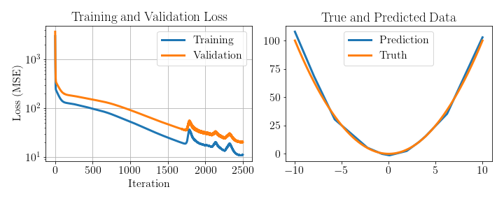
Let’s now try out our implementation on a toy problem where we want to approximate the ground truth function \(f^{*}(x) = x^2\). We’ll generate a dataset of 1000 training and test examples and use a network with 15 hidden nodes. For training we’ll use a learning rate lr = 1e-3 and epochs = 2500.
1
2
3
4
5
6
7
8
9
10
11
12
13
14
15
16
17
 # Instantiate network with 15 hidden nodes
nn = TwoLayerNetwork(1, 15, 1)

# Generate training and test data
ntrain = 1000
Xtrain = 5*np.random.randn(1, ntrain)
ytrain = Xtrain * Xtrain

ntest = 1000
Xtest = np.linspace(-10, 10, ntest).reshape((1, ntest))
ytest = Xtest * Xtest

# Train the network
loss = nn.train(Xtrain, ytrain, 1e-3, 2500)

# Get the prediction on the test data
ypred = nn.predict(Xtest)
The results are shown below. We indeed see that both the training and validation loss decrease over time and that the validation loss is only slightly higher than the training loss. For the plot on the right we see the predictions from the test data closely match the ground truth function. Code to generate this plot and run this example can be found in this notebook.